ECON 201B - Microeconomic Theory: Basic Concepts and Techniques of Noncooperative Game Theory and Information Economics

Winter 2026, Tomasz Sadzik

This is the second course in the PhD microeconomics sequence at UCLA. The topics covered are static games, Nash equilibrium concepts, dynamic games, and applications (Bertrand, Cournot, Hotelling, auctions, Stackelberg, bargaining, reputation, signaling, cheap talk). We follow loosely Mas-Colell, Whinston, and Green. Please let me know at kennyguo@ucla.edu if you spot any errors. Thanks!

Problem Set Solutions:

• Problem Set 1 (games, strategies, rationalizability)
• Problem Set 2 (weak dominance, nash equilibria, mixed NE)

Problem Set 1: Games, Strategies, and Rationalizability

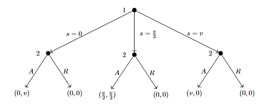
1. Ultimatum Game. Consider the following game. Two players, 1 and 2, bargain to determine the split of \(v\). Bargaining works as follows. Player 1 offers a split, \(s\), which must take one of the following three values: \(0\), \(v/2\), or \(v\). Player 2 observes this offer, and either accepts or rejects it. If 2 accepts the offer, 1 gets a payoff of \(s\), and 2 gets a payoff of \(v-s\). If 2 rejects the offer, both players get \(0\), and the game ends.

1. Draw the extensive form of this game.
2. Determine the strategy sets for each player in this game.
3. Draw the normal form for this game.
4. Identify any strictly dominated strategies. What is left after iterative deletion of strictly dominated strategies?

Answer.

1. Let \(A\), \(R\) represent Accept and Reject. The extensive form tree is given below.

2. The strategy set for player 1 is \(S_1 = \{0, v/2, v\}\). The strategy set for player 2 is conditional on that of 1: \(S_2 = \{(X\mid0, Y\mid\frac{v}{2}, Z\mid v) \, : \, X,Y,Z \in \{A, R\}\}\). Expanded out fully and omitting conditional notation, we have \[ S_2 = \{(A,A,A), (A,A,R), (A, R, A), (A, R, R), (R, A, A), (R, A, R), (R, R, A), (R, R, R)\}.\]

3. The normal form game matrix is given below.

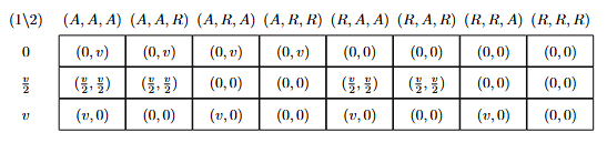
4. No strategy of Player 1 is strictly dominated (e.g. fix Player 2’s strategy to \((A,R,R)\). No mixture of the other two strategies has strictly greater payoff than the third for Player 1, as they are all \(0\)). Likewise, no strategy of Player 2 is strictly dominated (e.g. fix Player 1’s strategy to \(v\). All strategies give payoff of \(0\) for Player 2). Thus, the entire strategy profile of both players is left after IDSDS.

2. Cournot Limit. Recall that we claimed the linear Cournot game with 2 firms is dominance solvable. Given that the \(1\)-rationalizable set is \([0, \gamma(0)]\), the \(2\)-rationalizable set is \([\gamma^2(0), \gamma(0)]\), the \(2\)-rationalizable set is \([\gamma^2(0), \gamma^3(0)]\), etc., prove that this converges to a point. Compute what this limit is.

Proof.

Recall the linear Cournot game is given by \[\begin{align*} q &= q_1 + q_2, \\ p(q) &= a - bq, \, a, b \geq 0, \\ c_i(q_i) &= cq_i, \, i = 1,2, \, c \geq 0, \end{align*}\] utilities are given by profit, and where \(q_1, q_2 \geq 0\), \(b \neq 0\). The best-response function \(\gamma\) for both firms is then given by \[ \gamma(q_{-i}) = \max\left\{\frac{a-c}{2b}-\frac{q_{-i}}{2}, 0\right\} \] It can be shown that if \(q_{-i} \in [\underline{q}, \overline{q}]\), then all \(q_i < \gamma(\overline{q})\) and all \(q_i > \gamma(\underline{q})\) are strictly dominated. With this fact, we see how the strategy sets (which start as \([0, \infty)\)) for both players follow the sequence above. Observe that the lower bounds follow the subsequence \((\gamma^{(2t)}(0))_{t\geq 0}\) while the upper bounds follow the subsequence \((\gamma^{(2t + 1)}(0))_{t\geq 0}\). Without loss of generality, assume \(a-c > 0\) (if not, the strategy sets trivially converge to \(\{0\}\)). We then note that \[ \gamma^{(t)}(0) = -\left(\frac{a-c}{b}\right)\sum_{s=1}^t\left(-\frac{1}{2}\right)^s \] which converges as \(t \rightarrow \infty\) by the alternating series test. Thus, the limit is unique, meaning \(\lim_t \gamma^{(t)}(0) = \lim_t \gamma^{(2t)}(0) = \lim_t \gamma^{(2t + 1)}(0)\). The strategy sets become singletons after IDSDS, so the game is dominance-solvable. Computing this limit, we find: \[\begin{align*} \underset{t\rightarrow \infty}{\lim} \gamma^{(t)}(0) &= -\left(\frac{a-c}{b}\right) \sum_{s=1}^\infty \left(-\frac{1}{2}\right)^s \\ &= -\left(\frac{a-c}{b}\right)\sum_{u=1}^\infty \left(-\frac{1}{2}\right)^{2u-1}+\left(-\frac{1}{2}\right)^{2u} \\ &= -\left(\frac{a-c}{b}\right)\sum_{u=1}^\infty -\frac{2}{2^{2u}} +\frac{1}{2^{2u}} \\ &= \left(\frac{a-c}{b}\right)\sum_{u=1}^\infty \frac{1}{4^{u}} = \boxed{\left(\frac{a-c}{3b}\right)} \end{align*}\]

3. Asset Bubble. Imagine a game with \(I\) investors, each of whom owns one unit of stock. Each of them bought it at time zero, for zero dollars (which is a normalization). The value of the asset keeps rising one dollar per day. The strategy of each investor \(i \leq 100\) is to pick a day in the set \(\{1, 2, \ldots, 100\}\) when \(i\) sells the asset. We will model this as a Normal form game (each investor makes the decision at time zero, leave the instructions to an associate, and leaves for long holidays). The price of the asset works as follows. If \(n\) is the first day when anyone sells the asset, the price this day will be \(n\) divided by the number of traders that chose to sell that day. Each day afterwards, the asset price is zero. Finally, and investor incurs a cost of holding the asset. The total cost is \(\varepsilon > 0\) times the day at which the investor sells the asset. The payoff to investor \(i\) is the price at which \(i\) sold the asset minus the cost of holding the asset.

1. Show which strategies for an investor are dominated.
2. Find the set of rationalizable strategies for an investor.

Answer.

1. Suppose investor \(i\) sells on day \(100\). If everyone else sells on day \(100\), \(i\)’s payoff is \(100/I - 100\varepsilon\). If the others follow any other joint strategy (i.e. there is at least one investor that sells before day \(100\)), \(i\)’s payoff is \(-100\varepsilon\). Now, consider investor \(i\) selling on day \(99\). If everyone sells on day \(100\), \(i\)’s payoff is \(99 - 99\varepsilon\), which is strictly greater than before (assuming \(I \geq 2\)). With the other investors following any other joint strategy, \(i\)’s payoff is \(-99\varepsilon\), which is strictly greater than \(-100\varepsilon\). Thus, selling on day \(100\) is dominated by selling on day \(99\). Note that we can only eliminate day \(100\) from the \(1\)-rationalizable set. For example, if \(2 \leq n < 100\), then a joint opponent strategy which would break the dominance of selling on \(n-1\) over selling on \(n\) would be all other investors selling on day \(100\) (assuming \(\varepsilon\) is small).

2. However, continuing the process of IDSDS, we can continue to eliminate the last day of selling from our rationalizable sets. This means this game is dominance-solvable, resulting in the unique singleton rationalizable strategy of all players which is to sell immediately on day \(1\).

4. Bertrand with Differentiated Products. Consider the following Bertrand competition with differentiated products. There are two firms in the industry. Each chooses a positive price for its product, and demand for product \(i\) as the function of the two prices is \(q_i = A - Bp_i + Cp_j\), where \(A,B \geq 0\) and \(C \in \mathbb{R}\) (if \(C>0\), \(i\) and \(j\) are substitutes, and if \(C <0\), they are complements, with the magnitude representing the strength of the relationship). The costs of each firm are normalized to zero, so the payoffs are the revenues. The action set of each firm is a set of prices in \([0, M]\).

1. For fixed \(A, B\), describe the set of strategies that are not dominated, as a function of \(C\).
2. For fixed \(A, B\), describe the set of strategies that survive the process of IDSDS, as a function of \(C\).

Answer.

1. The utility of firm \(i\) is given by \(u_i(p_i, p_j) = Ap_i - Bp_i^2 + Cp_ip_j\). Fixing a \(p_j\), we use the FOC to find the best-response function \(p_i^\star(p_j) = \frac{A}{2B} + \frac{Cp_j}{2B}\). Since the strategy set of \(j\) is \([0,M]\), this means the set of strategies that are not dominated for \(i\) is \([\frac{A}{2B}, \frac{A}{2B} + \frac{CM}{2B}]\cap[0,M]\) if \(C > 0\), or \([\frac{A}{2B} + \frac{CM}{2B}, \frac{A}{2B}]\cap[0,M]\) if \(C < 0\).

2. We consider three cases:

Case 1: \(\frac{C}{2B} \geq 1\). Continuing the IDSDS using the best-response function, we have the upper bound of the rationalizable set is \(M\), while the lower bound follows the diverging sequence \(\left(\frac{A}{2B}\sum_{s=0}^t\left(\frac{C}{2B}\right)^s\right)_{t \geq 0}\). Since the strategy set is bounded by \(M\), the unique rationalizable strategy is \(M\) for both firms.

Case 2: \(\frac{C}{2B} \leq -1\). Using (a) (\(C <0\)), it holds that the 1-rationalizable set is \([0, \frac{A}{2B}]\). Iterating again with the best response function yields the same interval, so the set of rationalizable strategies is \([0, \frac{A}{2B}]\).

Case 3: \(1 > \frac{C}{2B} > -1\). If \(I_k = [\underline{i_k}, \overline{i_k}] \cap [0,M]\) is the interval after the \(k\)-th deletion, then \(I_{k+1} = [\frac{A}{2B} + \frac{C\underline{i_k}}{2B}, \frac{A}{2B} + \frac{C\overline{i_k}}{2B}] \cap [0,M]\). Computing the length of the untruncated \(I_{k+1}\), we get: \[ \left|\frac{A}{2B} + \frac{C\overline{i_k}}{2B} - \frac{A}{2B} - \frac{C\underline{i_k}}{2B}\right| = |\frac{C}{2B}||\overline{i_k} - \underline{i_k}| < |\overline{i_k} - \underline{i_k}| \] so the interval strictly decreases in length, and thus converges to a point. This point must be a fixed point of the best response function, i.e. \[ p_i = \frac{A}{2B} + \frac{Cp_i}{2B} \,\,\,\,\,\, \text{which gives} \,\,\,\,\,\, p_i = \frac{A}{2B-C}. \] Since \(C < 2B\), this point is always positive, but can extend beyond the bound of \(M\). Thus, the unique rationalizable price for both firms is \[ \min\left\{\frac{A}{2B-C}, M\right\}. \]

Problem Set 2: Weak Dominance, Nash Equilibria, Mixed Nash Equilibria

1. A Game. Consider the following game in normal form, where Player 1 chooses rows and Player 2 chooses columns. In each cell, 1’s payoff is listed first and 2’s payoff second. \[\begin{array}{c|ccccc} & a & b & c & d & e \\ \hline A & (2,1) & (4,2) & (1,0) & (10,3) & (2,4) \\ B & (6,10) & (2,20) & (0,10) & (7,15) & (0,18) \\ C & (5,0) & (0,0) & (3,3) & (5,0) & (0,1) \\ D & (8,1) & (2,4) & (0,0) & (5,1) & (4,2) \\ E & (1,3) & (2,6) & (0,4) & (8,5) & (1,3) \end{array} \]

1. Does either player have strictly dominated strategies? If so, what are they? Does either player have weakly dominated strategies? If so, what are they?
2. What strategies are eliminated through iterative deletion of strictly dominated strategies? Is the game dominance solvable?
3. Completely characterize the set of pure-strategy Nash equilibria for this game.
4. Completely characterize the set of rationalizable strategies for this game.

Answer.

1. For player 1: \(E\) is strictly dominated by \(A\). \(B\) is strictly dominated by \(0.5A + 0.5D\). For player 2, \(a\) is strictly dominated by \(0.75(b) + 0.25(c)\). Besides the strictly dominated strategies, there are no additional weakly dominated strategies for either player.

2. After IDSDS, we have \(S_1'=\{A, C, D\}\) and \(S_2' = \{b,c,e\}\). \(d\) becomes strictly dominated after we eliminate \(E\) from Player 1’s set after the first round (it was originally a best-response to a mixed belief of \(A\) and \(E\)).

3. There exists one unique pure strategy equilibrium: \((C, c)\).

4. We have that a strategy is rationalizable if and only if it surives IDSDS. Thus, the rationalizable strategies are the ones listed in part (b).

2. Location Choice. Consumers are uniformly distributed along a boardwalk of length 1 mile. The price of ice cream is fixed by a regulator, so consumers go to the nearest firm because they dislike walking (assume that at the regulated price all consumers will purchase an ice-cream cone even if they have to walk a full mile). If more than one vendor is at the same location, they evenly split the business.

1. Consider a game where two ice-cream vendors pick their locations simultaneously. Show that there exists a unique pure-strategy Nash equilibrium.
2. Show that with three vendors, no pure-strategy Nash equilibrium exists.

Proof.

1. Without loss of generality, let the two vendors be \(A\) and \(B\), let each of their strategy sets be \(a,b \in [0,1]\) (the location they choose), assume price is one, and assume unit density of consumers (i.e. a region of length \(x\) amounts to \(x\) units of demand). We show that \((0.5, 0.5)\) in the unique NE. By symmetry, we only consider the case where \(A\) deviates. If \(a < 0.5\), then demand for \(A\) falls to \(a + (0.5-a)/2 < 0.5\), the demand at \((0.5, 0.5)\). Similarly, if \(a > 0.5\), then demand for \(A\) falls to \((1-a) + (a-0.5)/2 < 0.5\), the demand at \((0.5,0.5)\). Price is fixed, so any deviation yields strictly lower profit, meaning both vendors are best-responding to each other.

Now suppose there’s another NE. * Case 1: \(a \neq b\). Without loss of generality, assume \(a < b\). Consider vendor \(A\) and deviation \(a' = (a + b)/2\). \(A\) now captures \((a+b)/2 + ((a+b)/2 + b)/2\) demand, which is strictly greater than the \((a+b)/2\) demand before. Thus, \(a \neq b\) cannot be a NE. * Case 2: \(a = b \neq 0.5\). Consider when \(a = b > 0.5\) (the other case is analogous). Both vendors split the market and get \(0.5\) demand each. Consider the deviation of \(A\) to \(a' = (a + 0.5)/2\). Now, \(A\) captures \((a+0.5)/2 + ((a+0.5)/2 + b)/2\) demand, which is strictly greater than \(0.5\) from before. Thus, Case 2 cannot be a NE.

2. Let the vendors be \(A, B\), and \(C\). Suppose that \((a, b, c)\) is a NE. We have the cases:

• Case 1: \(a=b=c\). Thus, demand is split \(1/3\) for each firm. If \(A\) deviates towards \(1/2\) (or if at \(1/2\), away by a small amount \(\varepsilon\)), \(A\) can capture demand greater than \(1/3\), so not a NE.
• Case 2: \(a,b \neq c\). Without loss of generality on the ordering of the players and the \(>\) versus \(<\), assume \(a \leq b < c\). \(C\) can thus move to \((b+c)/2\) and capture more demand, so not a NE.

These cases (when generalized) cover all potential pure strategy profiles, so no pure-strategy NE exists.

3. Costly Bids. Two risk-neutral firms, \(i = 1,2\), produce a homogeneous product at a unit cost \(c > 0\). There is a single consumer who buys either one unit of the good or nothing. The consumer has a reservation value \(v > c\), and resolves indifference in favor of purchasing at price \(p = v\).

Suppose the firms simultaneously decide whether to announce prices \(p_i \geq 0\). If a firm chooses to quote a price, it incurs a cost \(k > 0\) (e.g., to pay a salesperson to visit the buyer), but it has the option not to quote a price (saving the cost \(k\)). Suppose \(0 < k < v - c\).

The consumer buys the good at the lowest available price (provided it does not exceed \(v\)), and chooses between the firms with equal probabilities in the event of a tie.

1. Does this game have a pure-strategy Nash equilibrium? Justify your answer.
2. Characterize the symmetric mixed-strategy Nash equilibrium.

Answer.

1. It doesn’t. Suppose there exists some pure-strategy NE. We consider the cases:

• Case 1: Both firms quote a price. Both prices should be at least \(c + k\) to cover for the cost of production and quoting, if their good is purchased. If one firm is priced differently from the other, the firm who’s pricing lower has incentive to unilaterally raise by \(\varepsilon\), still under the other firm’s price, and claim strictly higher profit. If both firms set prices equal, but both strictly greater than \(c+k\), then one firm has incentive to undercut by a very small \(\varepsilon\), still above \(c+k\), to claim the buyer’s demand entirely, rather than face the coin toss. Finally, note that both firms pricing exactly at \(c+k\) is not stable, because the expected profit would be negative (half chance consumer buys from them and they get 0 profit, half chance consumer doesn’t and they pay \(k\), so \((0.5)(c+k-c-k)+(0.5)(-k)\)), and neither firm can undercut anymore without suffering negative profit, so a firm would want to unilaterally deviate to not quoting. Both firms would therefore have to set equally their prices at least at \(c+2k\) to make the expected profit nonnegative, however, as stated before, one firm can then slightly undercut.
• Case 2: One firm quotes, the other doesn’t. In this case, the quoting firm has a monopoly and can price their good at \(v\) (which is strictly above \(c+k\) by assumption). However, the non-quoting firm now has an incentive to quote at \(v-\varepsilon\), still above \(c+k\), giving strictly positive profit.
• Case 3: Both firms stay out of the market. Clearly, one firm has an incentive to quote at \(v\) which has strictly positive profit.

Thus, there does not exist a pure strategy NE.

2. First note that a firm not quoting is chosen with positive probability, i.e. it is a best response to some other action. To see this, let \(F(p)\) characterize the CDF of a firm over prices, given the firm quotes a price. If \(p\) is high enough to where \(F(p)\) is very close to \(1\), the expected profit in a symmetric mixed NE, , is \[\underbrace{(1-F(p))}_{\mathbb{P} \text{ that you win}}\cdot (p-c) - k < 0,\] which is strictly worse than not quoting (gives payoff of \(0\)). Thus, let \(0 < q < 1\) be the probability a firm quotes a price.

We also note that the support of this CDF is from \([c+k, v]\). Pricing above \(v\) would result in a strictly negative payoff (\(-k\)), and pricing below \(c+k\) would result in a strictly negative payoff (since it costs \(c+k\) to sell), so they are not best-responses to any other action. However, pricing within \([c+k, v]\) are best-responses, namely, pricing within \((c+k,v]\) is a best-response to the other firm not quoting, and pricing at \(c+k\) is a best-response to the other firm pricing at \(c+k+\varepsilon\).

Thus, we now turn to pinning down \(q\) and \(F(p)\). In a symmetric mixed NE, each action should yield the same expected profit (namely, \(0\), since not quoting yields deterministic \(0\) profit). Particularly in the event of quoting, any \(p\) quoted must satisfy in the symmetric mixed NE \[ \begin{align*} 0 &= \underbrace{(1-q)\cdot(p-c)}_{\text{Monopoly}} + \underbrace{q\cdot\left( F(p)\cdot 0 + (1-F(p))\cdot (p-c)\right)}_{\text{Both Quote}} - k \\ &= (1-q\cdot F(p))(p-c) - k. \end{align*} \] Rearranging gives \[ F(p) = \frac{p-c-k}{q(p-c)}. \] By CDF, we know \(F(v) = 1\), so solving for \(q\), we get \[ 1 = \frac{v-c-k}{q(v-c)} \implies q = \frac{v-c-k}{v-c}. \] Thus, the symmetric mixed NE is characterized by \(q^\star = \frac{v-c-k}{v-c}\) and \(F(p) = \frac{(p-c-k)(v-c)}{(v-c-k)(p-c)}, \, p \in [c+k, v]\).

4. Clinching Auction. The following is a generalization of the standard English auction to a setting with multiple identical goods (due to Ausubel, 2004). Imagine that a seller has two copies of a good to sell. There are two potential buyers, \(i = 1,2\), and buyer \(i\) has a value \(v_i^1\) from owning one unit, and \(v_i^1 + v_i^2\) from owning two units. We assume that marginal utilities are decreasing and bounded: \[ 0 \leq v_i^2 \leq v_i^1 \leq 1000, \] and that all values and marginal values are integers.

The auction is indexed by price \(p\), which starts at 0 and increases by one unit in every round. In each round, each player announces their demand at the given price. A player the first unit at a price at which the other player’s demand drops below 2 (i.e., the number of goods available to a player is \(2\) minus the goods demanded by the other player), and pays the corresponding per-unit price.

The price continues to rise, and at some price the second unit is clinched (either by the player who already bought the first unit or by the other player). At this point the game ends. If both players drop their demands at the same time, ties are broken by a coin toss. If a player is indifferent between buying and not buying at some price, assume they choose to buy.

1. First, think about the game as a static game. Each bidder \(i\) submits a demand function consisting of two numbers (marginal utilities) \((b_i^1, b_i^2)\) such that \[0 \leq b_i^2 \leq b_i^1 \leq 1000.\] Payments are computed by running the auction using these bids. Show that submitting truthful bids, \[b_i^1 = v_i^1, \quad b_i^2 = v_i^2,\] is weakly dominant.

2. Now consider the dynamic version of the auction. Identify some strategies that are weakly dominated.

3. In the dynamic game, is truthful bidding weakly dominant? Justify your answer.

Proof.

1. Suppose you submit non-truthful bids. Clearly, bidding higher than your true marginal utilities is weakly dominated, so we consider the cases:

• Case 1: \(b_i^1 = v_i^1, \, b_i^2 < v_i^2\). Then consider if \(j\) has \(b_i^2 < b_j^2 \leq v_i^2\), ceteris paribus. \(j\) then clinches the first unit, but had you bid truthfully, you would’ve clinched the first unit at a strictly positive (expected) surplus. If \(j\) bids at or below your lowered \(b_i^2\), the payoff is better or the same compared to if you had bid truthfully. If \(j\) bids above \(v_i^2\), \(j\) would clich the first item and you would receive \(0\) payoff, whether you bid truthfully or below. Thus, this case is weakly dominated by bidding truthfully.
• Case 2: \(b_i^1 < v_i^1, b_i^2 = v_i^2\). Again, consider if \(b_i^1 < b_j^1 \leq v_i^1\), ceteris paribus. \(j\) then clinches the second unit, but had you bid truthfully you would’ve clinched the second unit as a strictly postive (expected) surplus. The reasoning follows as before, and this case is weakly dominated.
• Case 3: \(b_i^1 < v_i^1, b_i^2 < v_i^2\). This is a combination of the two previous cases. For example, \(j\) could bid \(b_i^1 < b_j^1 \leq v_i^1\) and \(b_i^2 < b_j^2 \leq v_i^2\), to which bidding truthfully would give strictly positive (expected) profit.

Thus, truthful bidding is weakly dominant.

2. Clearly, bidding strictly above your value, say for the second good, is weakly dominated by bidding at your true value for that good. If \(j\) decides to bid above you, both cases net you \(0\) profit. Yet if \(j\) bids below you, you clinch the second item, but at negative utility, rather than a always non-negative utility at truthful bidding. If \(j\) bids the same as you (both of you drop out as the same time), if you clinch from the coin toss, your utility is negative, and if you don’t, your utility is \(0\). In any case of what \(j\) does, jumping out as soon as the price rises above your true value weakly dominates staying in.

3. No, as it isn’t weakly better than every other bid facing any opponent strategy, namely, the opponent strategies can now be conditional on what happened in previous price hikes. Suppose I have \(v_i^1 = v_i^2 = 10\) and the price is still at \(p=2\). However, suppose opponent \(j\) takes the strategy of staying in the auction forever if I demand \(2\) units at \(p=2\), or dropping out of the auction at \(p = 3\) if my demand drops to \(1\) at this price, i.e., I set my \(b_i^2 = 1\). Then for me, bidding truthfully would net \(0\) utility, but if I bid untruthfully (\(b_i^2 = 1\)), \(j\) would clinch the first unit, but I would clinch the second unit, netting \(10 - 3 = 7\) utils. Thus, truthful bidding is not weakly dominant.